Where I explore filters in electronics and use the Espotek Labrador to demonstrate how to understand filters and create amplitude response curves. This discussion will be absurdly simplistic in comparison to the topic. My goal is to show sufficient theoretical examples of filters, so we can then test them using the Labrador.
Video: How to Use the Espotek Labrador to Analyze a High Pass Filter Amplitude Response Curve#
Our goal with the Labrador is to test the following filter analysis. Doing so will help make electronics more intuitive and familiar and help you understand as to how to use the Labrador. It will also help you understand how to plot data and in this case, using a log scale.
I highly encourage you to use this page, to:
Understand how to measure the amplitude response of a circuit using the Labrador
Analyze the measurements using Julia or Matlab (or Octave or gnuplot….) It is this second step that will help you to understand filter amplitude response curves.
MIT Lecture on Filters Very good introduction to filters. I like the instructor’s approach of helping you understand the behavior of resistors, inductors and capacitors to make educated guesses as to a circuit’s behavior.
A Basic Introduction to Filters Texas Instruments
An application note which describes filters and helps you to understand why filters are important and how to create them. I recommend, at a minimum, reading the first couple of pages.
A comment made by the instructor in the above recommended video “almost every electrical circuit has a filter.” This is the best reason as to “Why filters?”
The most simple and compelling filters are the decoupling capacitors on USB cables or the noise capacitors on power connections. Going up from there are the filters which are designed to eliminate a specific set of frequencies and focus on a desired frequency such as an AM radio tuner. There are cross-over networks in audio speakers which eliminate low frequency signals going to the treble amplification and eliminate high frequency signals going to the bass amplification.
The goal of any filter is to remove the unwanted frequencies to achieve the greatest utility in the band of the desired frequencies.
The goal in this discussion, isn’t to focus on a specific application of filters as it is to understand a filter’s amplitude response curve. This discussion will help you to understand how specific combinations of resistors, inductors and capacitors will have a particular response. Which in turn, will help you to understand how a circuit will behave when driven with a specific frequency.
Similar to the instructor’s approach in the video, let’s remember the behavior of a resistor, inductor and capacitor with a DC signal, a low frequency AC signal and a high frequency AC signal:
Device
DC
Low Frequency AC
High Frequency AC
Resistor
Linear
Linear
Linear
Capacitor
Open Circuit
Open Circuit
Short Circuit
Inductor
Short Circuit
Short Circuit
Open Circuit
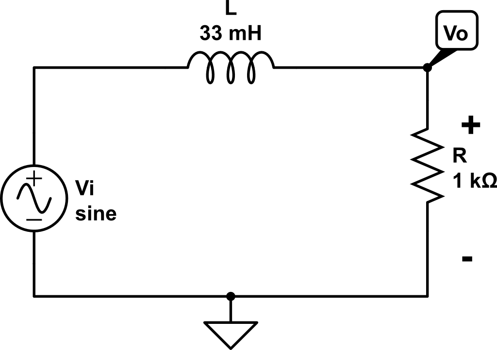
Let’s start with a theoretical approach by using CircuitLab. With CircuitLab, you quickly create a circuit such as this one:
LR Circuit for a low pass filter
And run a Frequency-Domain Simulation to understand its Amplitude Response Curve. In this graph, we are showing the relationship between Vi and Vo. To smooth it out and make the curve more understandable, the practice is to plot using a log scale, instead of a linear scale.
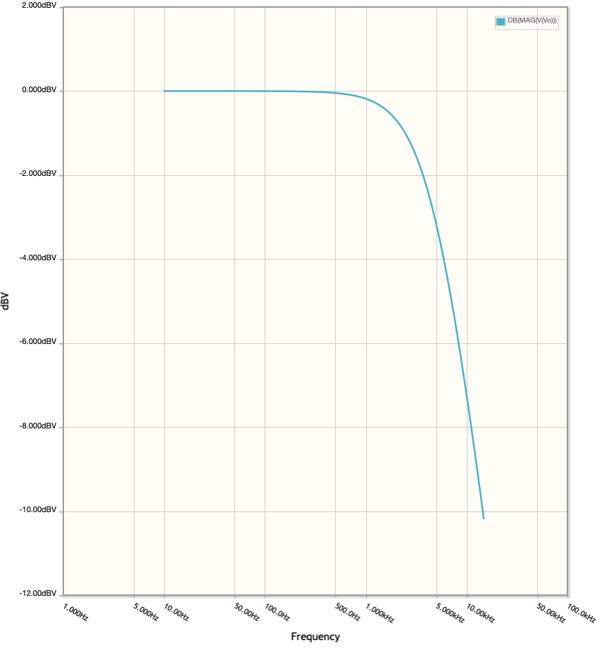
Amplitude Response for LR Circuit for a low pass filter
This graph is showing the ratio between Vo and Vi is 1 (Vo = Vi) at low frequencies and it declines as the frequency increases (Vo -> 0). Let’s make a similar table as above to reflect the circuit: (note: remember the plot is the magnitude of Vo/Vi, so its unsigned)
Device
DC
Low Frequency AC
High Frequency AC
1kΩ Resistor
Vr = -Vi
Vr = -Vi
Vr -> 0
33 mH Inductor
Vl = 0
Vl = 0
Vl -> infinity
LR Circuit
Vo/Vi ≅ 1
Vo/Vi ≅ 1
Vo/Vi -> 0
To understand this response, first examine this circuit as a voltage divider at DC and low frequencies (first two columns).
Vl (the voltage across the inductor) is approximately 0.
Which means the voltage, Vo, is equal to the voltage across the resistor, Vr.
Apply Kirchoff’s law:
Vi - Vo = 0
Vo = Vi
Vo/Vi = 1.
Then make similar assumptions at high frequencies. As the frequency increases, the inductor acts like an open circuit. Which means the current through the resistor goes to zero, making Vo very small, in turn reducing the ratio to a very small number (goes to zero).
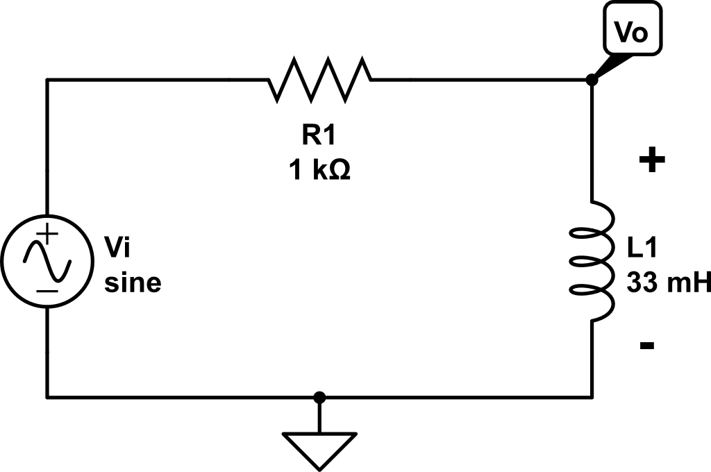
Now let’s switch the position of the inductor and the resistor and the behavior is:
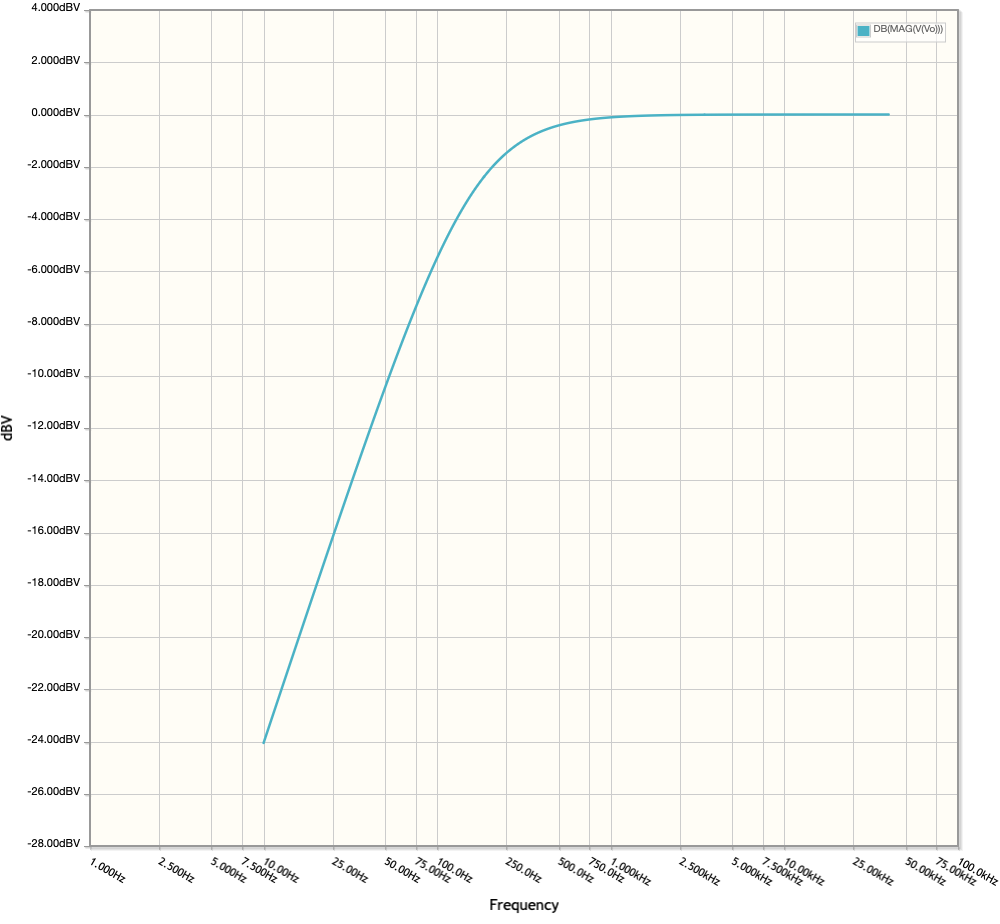
RL Circuit for a high pass filter
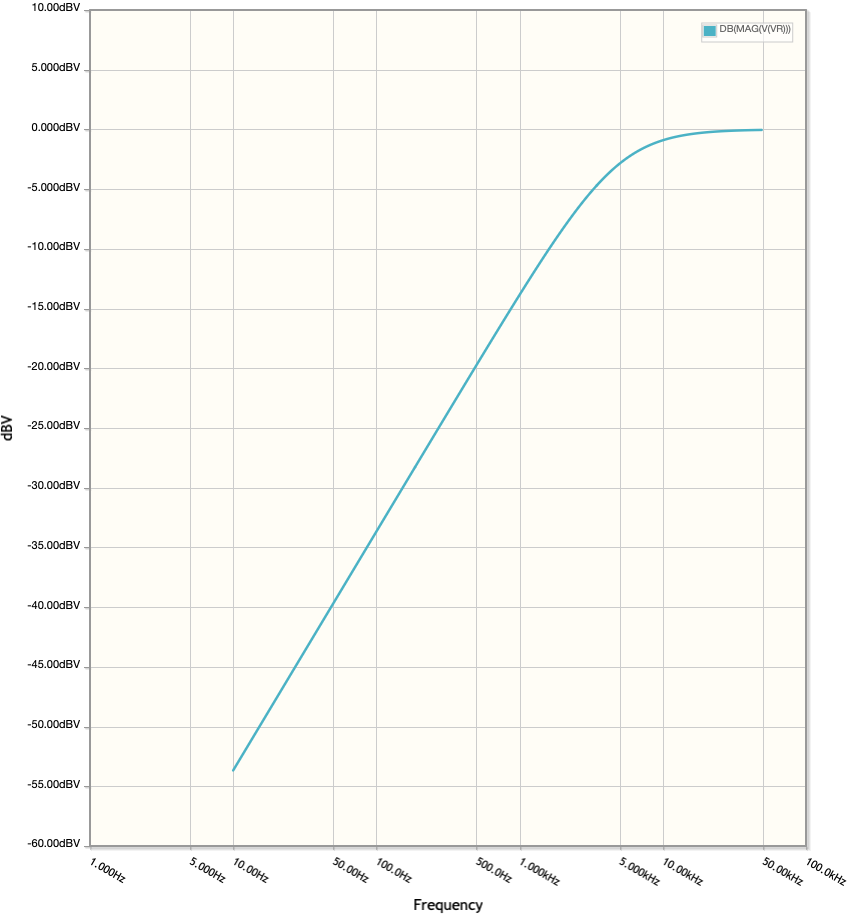
Amplitude Response for RL Circuit for a high pass filter (10Hz - 50kHz)
(We will analyze this circuit using the Labrador.)
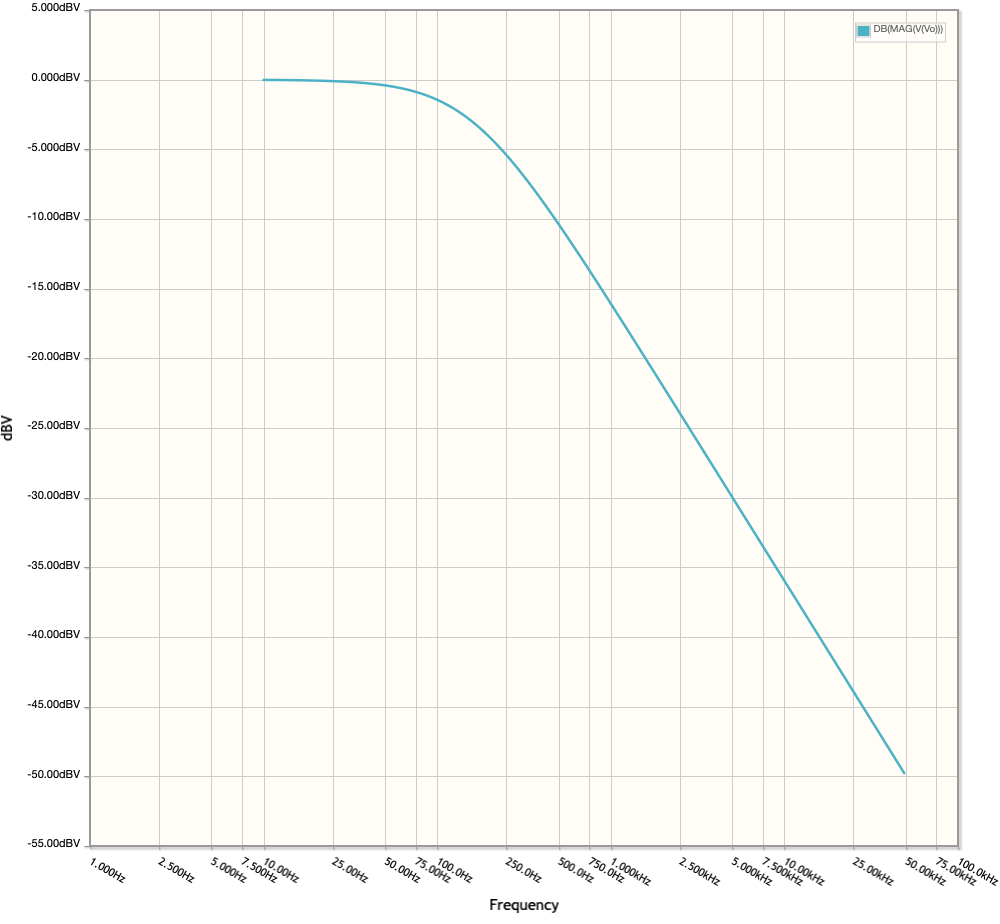
And finally, replace the inductor in the first circuit with a capacitor and we have a high pass filter (again), however it has a dramatically different curve.
Amplitude Response for CR Circuit for a high pass filter (10Hz - 50kHz)
Note how the curve begins to break a little over 100Hz and is halfway at 250Hz. While the RL circuit curve begins about 2.5kHz and halfway is about 5kHz. The curve themselves exhibit a slightly, different curvature.
Finally, one more curve where we exchange the positions of the resistor and capacitor and achieve a low pass filter.
Amplitude Response for RC Circuit for a low pass filter (10Hz - 50kHz)
Before you start, its best to organize your data collection to make it easier to use for the second part of this expermint (Analyze the measurements). For Julia (or a Matlib equivilent), an array which looks like this will be a great way to record your data:
I recommend opening up a text file, pasting the above code then enter new data as you gather it. (Replacing the values that currently exist and follow the format of blanks between values and a “;” at the end of each line.)
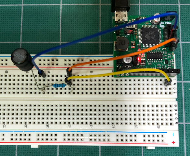
Build the simple RL circuit on the breadboard containing the Labrador.
Yellow wire - Signal Generator CH1 (DC) to first leg of 1k resistor
Orange wire - Oscilloscope CH1 (DC) to first leg of 1k resistor
Blue wire - Oscilloscope CH2 (DC) to second leg of 1k resistor
33 mH Inductor - one leg to second leg of resistor and second leg to ground
Open the Labrador application and:
Set the PSU to 8V (uncheck Lock PSU, move slider, then check Lock PSU)
Set Signal Gen CH1 Amplitude to 5V
Ensure Oscilloscope -> Show Range Dialog on Main Page is checked or press M
Vmax to 3V and Vmin to -3V
Check AC Coupled on Oscilloscope CH1 and check Trigger
If the top of CH1 is flat, check Paused then uncheck Paused (see Software Bug)
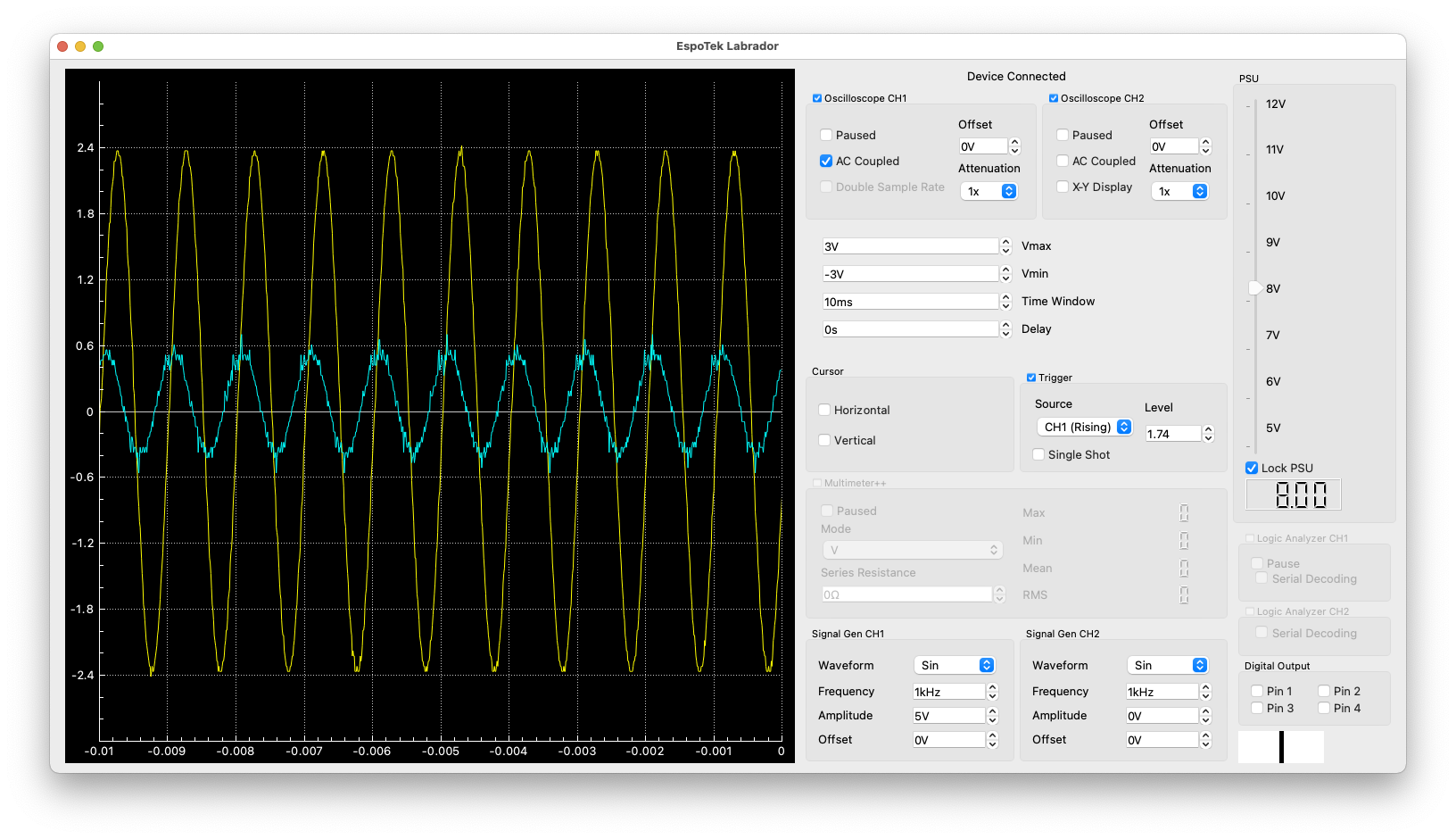
Check Oscilloscope CH2 and if all went well, you will have this image:
Labrador application showing initial results at 1kHz
Now we are ready to take measurements.
Set the Frequency input on Signal Gen CH1 to 50Hz
Change the Time Window to 40ms to see several periods of CH1
Begin taking measuring the amplitude of both signals using the vertical cursors.
Click on the highest point of the CH1 signal then drag the dotted cursor to the lowest point. The delta V (ΔV) number will be the total amplitude. For CH1, it will be extremely close to 5V.
Note: Using the cursors to measure amplitude on the Labrador is one of its best features, the click and drag with a screen measurement is outstanding!
Going back to our comment at the start, let’s begin to enter data:
As you increase the frequency, you will need to adjust the time window so that only a few periods are shown in the window. This will allow you to get the best measurements.
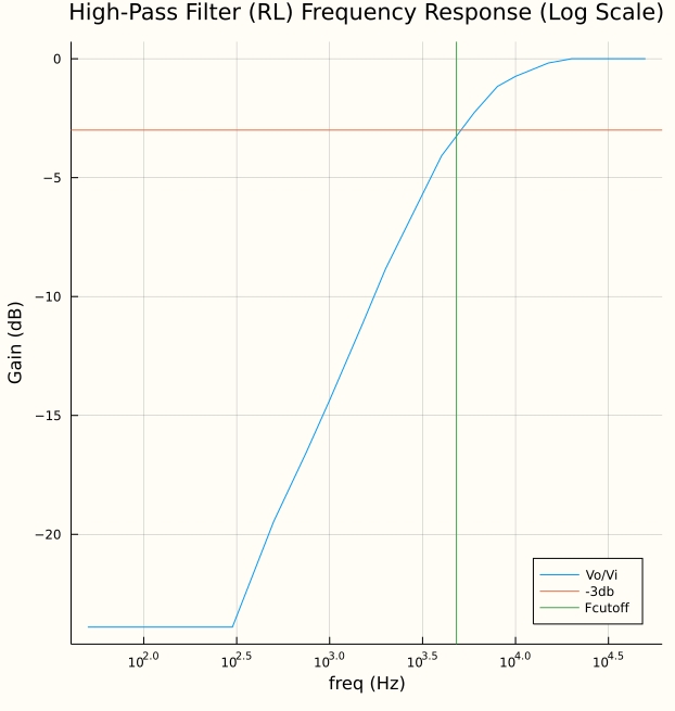
Now its time to view the data. I used this julia program to graph it:
Very similar to our theoretical analysis. Note the -3db horizontal line does intersect with the vertical line (Cutoff frequency) quite well on the graph.
I did spend some time looking at the graph and checking my measurements. When I first attempted the graph, it was quite rough as I didn’t take sufficient time in precisely measuring the amplitudes. It pays to be precise and patient when you are making measurements!
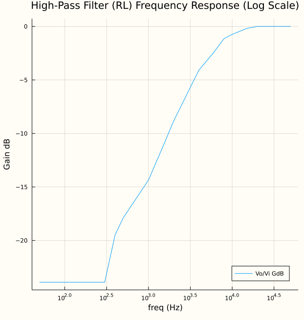
Here is a plot of the original data, which you can see above in step 4:
Original data (Step 4): Julia plot of RL Filter Amplitude analysis
Why was this important?
The goal of this experiment was to provide a general understanding of filters. By using the Labrador to confirm one of the filter designs, it helped us to feel comfortable making measurements using the Labrador, refine the measurements and graph them to compare to our theoretical results.